Populations grow when blank" rel="noopener noreferrer">births and immigration add individuals faster than deaths and emigration remove them. To answer 5.1 biology questions, use this births, deaths, immigration, and emigration framework to work out the change in population over time populations grow. That four-part accounting identity (births, deaths, immigration, emigration) is the core of every "5.1 how populations grow" lesson, and once you have it locked in, the rest of the chapter, including exponential growth, logistic growth, carrying capacity, and density dependence, flows directly from it.
5.1 How Populations Grow: Biology Answers and Models

Marcus Whitmore
1 Jun 2026

Population growth basics and the key drivers

Think of a population like a bank account. Money goes in two ways: deposits (births) and transfers in (immigration). Money goes out two ways: withdrawals (deaths) and transfers out (emigration). The balance at the end of the year is simply: population at time 2 = population at time 1 + (births minus deaths) + (immigration minus emigration). That's it. Every population model you'll encounter in a 5.1 lesson is built on that identity.
For a closed population, one with no migration, you only track births and deaths. The per-capita growth rate, often called r (the intrinsic rate of increase), is just the per-capita birth rate (b) minus the per-capita death rate (d): r = b − d. If r is positive, the population grows. If r is zero, it holds steady. If r is negative, it shrinks. Simple as that.
- Births (natality): new individuals added through reproduction
- Deaths (mortality): individuals permanently removed from the population
- Immigration: individuals moving into the population from elsewhere
- Emigration: individuals leaving the population for another area
- Net change per time step = (births − deaths) + (immigration − emigration)
Exponential vs logistic growth models
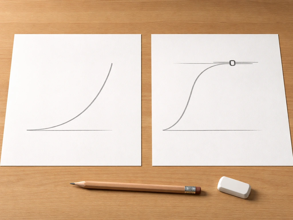
Exponential growth happens when r stays constant regardless of how many individuals are already in the population. No competition, no resource limits, no crowding. The equation is dN/dt = rN, meaning the rate of change in population size is just r multiplied by however many individuals exist right now. Because every individual keeps producing new individuals at the same rate, the curve bends upward steeply, like compound interest. You've probably seen this called a "J-shaped curve."
Logistic growth is what happens when you add reality. As the population grows, resources get tighter, space fills up, and the per-capita growth rate starts to drop. The logistic model introduces a ceiling called the carrying capacity (K), which is the maximum population size the environment can sustain. The equation becomes dN/dt = rN × ((K − N)/K). When N is tiny compared to K, that (K − N)/K term is close to 1 and growth looks nearly exponential. As N approaches K, the term shrinks toward zero and growth slows to a crawl. The result is the familiar S-shaped, or sigmoid, curve.
| Feature | Exponential Growth | Logistic Growth |
|---|---|---|
| Curve shape | J-shaped | S-shaped (sigmoid) |
| Per-capita growth rate (r) | Constant | Decreases as N increases |
| Upper limit on population | None | Levels off at K (carrying capacity) |
| Resource assumption | Unlimited | Limited by environment |
| Real-world applicability | Short bursts, ideal lab conditions | Most real populations over time |
| Key equation | dN/dt = rN | dN/dt = rN × ((K − N)/K) |
One thing students often miss: at N = K/2 (half of carrying capacity), logistic growth is actually at its fastest. That's the inflection point of the S-curve. Above that point, growth is still happening but decelerating. This matters for things like fisheries management, where harvesting a population near K/2 maximizes sustainable yield.
Birth–death processes and age/sex structure

A population isn't just a headcount. Who is in the population matters as much as how many. A population of mostly old individuals past reproductive age will shrink even if total numbers look reasonable. A population skewed heavily female will grow faster than one with many males, because reproductive output is tied to the number of reproducing females. That's why age structure and sex ratios belong in any serious "how populations grow" discussion.
Life tables are the standard tool for capturing this detail. A life table lists age classes (or life stages) and records, for each class: the probability of surviving to the next age (survivorship, often written as lx), and the average number of offspring produced per individual at that age (fecundity, written as mx or bx). When you multiply survivorship by fecundity across all age classes and sum them up, you get a value called R0, the net reproductive rate. If R0 is greater than 1, the population is replacing itself more than one-for-one and will grow.
Survivorship curves give you a visual summary of when mortality hits hardest. Type I curves (humans, elephants) show most individuals surviving to old age, then dying quickly. Type II curves (many birds) show a roughly constant death rate at all ages. Type III curves (most fish, insects, plants) show massive early mortality, with the few survivors living relatively long. The type of survivorship a population has dramatically affects how birth and death rates combine to drive overall growth.
Carrying capacity, limiting factors, and density dependence
Carrying capacity (K) isn't a fixed universal constant. It's a reflection of the current environment, specifically the limiting factors that cap how many individuals can be supported. Limiting factors include food availability, water, space, nesting sites, light (for plants), disease pressure, and predation. Change the environment and K changes with it. A drought lowers K for deer in a forest. Fertilize an algae tank and K shoots up temporarily.
Density dependence is the mechanism that actually enforces K. When population density rises above equilibrium, density-dependent processes kick in to bring it back down: birth rates fall (because there's more competition for mates and resources), death rates rise (because disease spreads faster in crowded conditions, predators have more prey to target, and food per individual drops). When density falls below equilibrium, the reverse happens. This feedback loop is what gives logistic growth its S-shape and what keeps most real populations from growing without limit.
Not all limiting factors are density-dependent. Density-independent factors, like a sudden hard frost, a hurricane, or a wildfire, can knock down a population regardless of how large or small it is. These produce sudden population crashes that aren't predicted by the smooth logistic model. Real populations live in the messy overlap of both types of regulation.
How to compute growth rates from real data

If you're given population sizes at two different times, you can estimate r for exponential growth directly. The relationship is N(t) = N0 × e^(rt), which rearranges to r = (ln N2 − ln N1) / (t2 − t1). In plain English: take the natural log of both population sizes, subtract them, and divide by the time elapsed. If you plot ln(N) on the y-axis against time on the x-axis, the slope of that line is r. A straight line confirms exponential growth; a curve that flattens out confirms logistic growth.
- Record population size (N1) at time 1 and population size (N2) at time 2
- Calculate the natural log of each: ln(N1) and ln(N2)
- Subtract: ln(N2) − ln(N1)
- Divide by the time interval (t2 − t1) to get r
- If r is positive and roughly constant across multiple time steps, growth is exponential
- If r decreases as N increases, the population is showing logistic (density-dependent) behavior
For life-table style problems, you'll usually be given a table of lx (survivorship) and mx (fecundity) values across age classes. Multiply lx by mx for each age class, then sum all those products to get R0. If R0 > 1, the population grows. If R0 = 1, it's stable. If R0 < 1, it declines. Some problems also ask you to estimate generation time (T), which is the average age at which individuals reproduce, weighted by their contribution to R0.
Practical scenarios: ideal lab conditions vs real ecosystems
In a controlled lab setting with unlimited food, space, and no predators, a bacterial culture or a population of fruit flies will follow exponential growth remarkably closely for a while. This is actually a useful teaching tool because it isolates the mechanics of birth and death without the noise of real-world limiting factors. Think of it like watching a sourdough starter double every few hours in perfect warmth with unlimited flour: the growth is real, but the conditions are artificial.
In a real ecosystem, those ideal conditions never last. A deer herd introduced to an island with no predators might show a J-curve for a few years, then crash hard when vegetation gets stripped bare. Classic studies, including Georgii Gause's work with Paramecium in lab dishes, showed the S-curve clearly: exponential early growth, a slowdown as resources thinned, and a plateau near K. Real ecosystems add predation, disease, seasonal variation, and competition, which means real population curves oscillate around K rather than sitting smoothly on it.
When you're working through a 5.1 problem that describes a "population in a new habitat with abundant resources," think exponential. When the problem mentions competition, disease, or the population approaching the environment's limit, think logistic. That framing alone gets you through most textbook questions correctly.
Impacts of density on resources, behavior, and survival
High population density doesn't just mean more individuals crammed together. It changes behavior, physiology, and survival in measurable ways. Locust swarms are a famous example: at low density, locusts are solitary and relatively calm. When density spikes, they switch to a gregarious phase, change body shape, and swarm in massive groups that strip vegetation. That behavioral switch is a direct response to crowding and is one of the most dramatic density-dependent effects in nature.
More commonly, high density increases competition for food and mates, slows individual growth rates (relevant for organisms that keep growing throughout life, like fish or trees), reduces immune function due to nutritional stress, and accelerates pathogen transmission. Each of these effects ultimately shows up as a change in birth rate, death rate, or both, which is exactly how density dependence feeds back into the population model.
At very low density, a different problem appears: the Allee effect. Populations can become so small that individuals struggle to find mates, cooperative behaviors break down, and inbreeding increases. Birth rates drop and death rates rise not because of crowding, but because of isolation. This is why conservation biologists worry about minimum viable population sizes, and it's a nuance worth knowing when you're thinking about what happens at the bottom of the logistic curve.
Biology answers to common misconceptions and how to check your reasoning
The most common mistake in 5.1 problems is confusing growth rate with population size. A population can be huge and still have a low or even negative growth rate. A tiny population can have a blazing-fast growth rate. Growth rate (r) describes how fast the population is changing right now, not how large it is. Keep those two things completely separate in your thinking.
Another frequent error is assuming populations always grow quickly. They don't. Most real populations spend a lot of time near K, fluctuating up and down in response to environmental variation. The J-curve is a special case that requires specific conditions (new habitat, abundant resources, no density-dependent pressure). If a problem gives you a stable, long-established population in a mature ecosystem, logistic thinking is almost always the right frame.
Students also sometimes forget that carrying capacity is not a hard wall. Populations routinely overshoot K, especially when there's a time lag between rising density and the feedback response (disease taking time to spread, for example). Overshoots are followed by crashes, which is why real population graphs look jagged rather than perfectly sigmoidal.
- Misconception: 'A bigger population always grows faster.' Reality: per-capita growth rate (r) can be the same or lower in a large population if density-dependent factors are operating.
- Misconception: 'Carrying capacity never changes.' Reality: K shifts with any change in limiting resources, climate, or habitat quality.
- Misconception: 'Exponential growth is the normal state.' Reality: exponential growth is a temporary phase; logistic growth is closer to the long-term norm.
- Misconception: 'Immigration and emigration don't matter much.' Reality: in fragmented landscapes, migration between patches can be the difference between local extinction and persistence.
- Misconception: 'Once a population hits K, it stops.' Reality: populations oscillate around K, often overshooting and crashing before settling.
Here's a quick self-check routine for any 5.1 problem: first, identify which of the four drivers (births, deaths, immigration, emigration) the problem is emphasizing. Second, ask whether the scenario suggests unlimited resources (exponential) or resource limits and competition (logistic). Third, check whether density-dependent effects are mentioned. If yes, expect birth rates to fall or death rates to rise as N increases. Fourth, if a number is given for population size and another for growth rate, make sure you're not treating them interchangeably. Work through those four steps and you'll catch the reasoning errors before they cost you on an exam.
If you're exploring this topic alongside related questions, like how to work through a specific answer key for a chapter 5 lesson 1 assignment, or you want a deeper dive into the mechanics of how real biological populations grow and what distinguishes them from idealized models, those threads connect naturally to everything covered here. The four-driver framework and the exponential-to-logistic progression are the backbone of population biology, and getting comfortable with them makes the rest of ecology significantly easier to navigate.
FAQ
How do I tell whether a population problem is using exponential or logistic growth when the wording is unclear?
Look for a cue that the per-capita growth rate changes with population size. If the problem says reproduction stays proportionally the same as numbers rise, it is exponential. If it mentions competition, limited resources, crowding, disease increase, or “approaching” a limit, it is logistic. When both are implied, decide based on whether the given data show a slowing relative growth rate (logistic) or a constant proportional rate (exponential).
If I’m given N1, N2, and time, how can I quickly check whether the growth is truly exponential?
Compute r using r = (ln N2 − ln N1)/(t2 − t1) and then see if the same r would work over another time interval if one is provided. Another practical check is to compare ln(N) values: exponential growth should produce a straight line trend in ln(N) versus time, while logistic growth makes that plot curve (flattening as N rises).
What’s the difference between “growth rate r” and “net reproductive rate R0,” and when does each matter?
r describes how fast population size changes per unit time (birth minus death effects, per capita), it is used in growth models like exponential and logistic. R0 summarizes population-level reproduction across age classes (from survivorship and fecundity), it is mainly for life-history and age-structured stability. A population can have R0 > 1 yet still show temporarily slower growth if deaths or resource limits affect r through time.
In logistic growth, why is the growth fastest at K/2, and what does that mean for exam problems?
The model’s growth term depends on N through (K − N), so when N increases from 0 to K/2 the “available room” is still large and growth accelerates. Past K/2, the (K − N) factor shrinks faster than the N factor increases, so net growth decelerates. On questions asking “when does sustainable yield peak,” it often corresponds to maximizing a birth-related or growth-related term, which is why K/2 is a common target.
Does logistic growth always mean births fall and deaths rise as the population approaches K?
In the simplest interpretation, yes, density dependence reduces per-capita birth and/or increases per-capita death as N increases. But exam questions may implement density dependence in only one demographic channel, such as a death rate term that rises with N while births stay constant. If only one driver is described to change with density, apply the density dependence only there.
Can a population overshoot carrying capacity K in logistic models?
Yes, overshoot can happen in real systems and sometimes in problems. The key idea is that feedback is not instantaneous. If density-dependent effects (like disease, food depletion, or predator response) take time to ramp up, N can temporarily rise above K, then crash when the delayed response catches up.
What is the Allee effect, and how is it different from “just logistic” growth at low density?
The Allee effect is a low-density failure mode where per-capita growth can be worse when N is small, due to difficulty finding mates or breakdown of cooperative behaviors. Logistic growth usually predicts near-exponential behavior at low N, not a strong decline in growth rate. In Allee scenarios, you may be asked about thresholds, extinction risk, or minimum viable population size.
Are density-independent factors always unrelated to density, and how do they change population graphs?
Density-independent factors act regardless of population size, like storms, hard frosts, or sudden habitat destruction. They can cause sharp drops, meaning the population curve can look jagged, with sudden crashes that logistic-only models do not predict. If a problem mentions abrupt environmental events, don’t assume smooth S-shaped recovery.
In a four-driver accounting identity, how do I handle immigration and emigration when they are given “per capita”?
Treat them as rates multiplied by the relevant population size, just like births and deaths. For example, immigration per capita adds I_rate × N individuals per time, and emigration per capita removes E_rate × N. Then use net change: (births − deaths) + (immigration − emigration) to update N.
How should I interpret age structure questions, especially when given l_x and m_x values?
Multiply survivorship to each age class by fecundity at that class, then sum across all age classes to get R0. If the problem also asks for generation time, the required weighting is tied to each age class’s contribution to reproduction, not just survivorship. A common mistake is to average ages using survivorship alone, instead of using reproduction-weighted contribution.
Why might a population have a low or negative r even if it has a large number of individuals?
Because r depends on the balance of per-capita births and deaths (and possibly immigration and emigration per capita), not on the absolute headcount. A large population can still be shrinking if deaths exceed births per individual, or if emigration and net losses dominate. That distinction is critical when problems ask for the direction of change rather than size.
If a problem describes a new habitat with abundant resources, when does the model stop being exponential?
It stops once density-dependent pressures emerge or resource limits become relevant. In practice, that means after the population has increased enough that competition, disease spread, or other limiting factors start to reduce the per-capita growth rate. If the scenario includes a time horizon or later observations, switch from exponential expectations early on to logistic-like slowing as N rises.
Next Article
5.1 How Populations Grow Answer Key Biology
Step-by-step biology answer key for 5.1 population growth: exponential vs logistic, carrying capacity, parameters, and c