Populations grow in biology when births and immigration add more individuals than deaths and emigration remove over a given time period. That net change can follow two main patterns: exponential growth, where numbers accelerate without any ceiling, and logistic growth, where expansion slows as the population approaches the maximum size the environment can support. Real populations almost always follow something closer to the logistic pattern, because food, space, and other resources are finite.
How Do Populations Grow in Biology: Models and Limits

Marcus Whitmore
5 May 2026

What "population" actually means in biology
In biology, a population is a group of individuals of the same species living in the same area at the same time and interacting with one another. That last part matters. A handful of frogs in one pond and another group of the same species in a pond ten miles away are typically treated as separate populations because they have limited contact. The key state variable biologists track is N, population size. Everything else, growth rate, resource use, age structure, builds on what N is doing over time.
Population growth is simply a change in N. If N goes from 200 to 240 individuals between spring and fall, the population grew by 40. If it drops from 200 to 160, it declined. Understanding why those numbers move requires looking at the four processes that drive every population on Earth.
The four engines of population change: births, deaths, immigration, emigration
Every change in population size comes down to a single accounting equation. Biology LibreTexts expresses it cleanly as: N(t+1) = N(t) + B(t) - D(t) + I(t) - E(t). Read it left to right: next period's population equals this period's population, plus births, minus deaths, blank" rel="noopener noreferrer">plus immigrants arriving, minus emigrants leaving. That's it. Four variables. If births and immigration outpace deaths and emigration, the population grows. If the reverse is true, it shrinks.
- Births (B): new individuals produced through reproduction within the population.
- Deaths (D): individuals lost to old age, predation, disease, accident, or starvation.
- Immigration (I): individuals moving into the population from somewhere else.
- Emigration (E): individuals leaving the population to settle elsewhere.
Immigration and emigration are easy to overlook, but they can be decisive. A small island population of birds can go locally extinct if emigration is high and immigration is blocked by geography. A recovering wolf population in a national park can rebound faster than birth rates alone predict if wolves disperse in from adjacent territories. When you're analyzing any real population, always ask whether movement is possible and how much of it is happening.
Two core models: exponential growth vs. logistic growth
Biologists use mathematical models to describe how N changes over time. Two models dominate introductory biology for good reason: they capture the two most important scenarios, unlimited resources and limited resources.
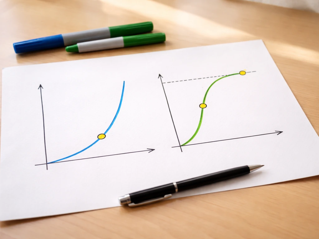
Exponential growth: the J-curve

Exponential growth happens when each individual contributes a constant rate of net new individuals regardless of how crowded the population gets. The continuous-time version is written as dN/dt = rN, where r is the intrinsic rate of natural increase (births minus deaths per individual per unit time) and N is current population size. Because r is multiplied by N, a bigger population produces even more new individuals, which makes the population bigger still. The result on a graph is a J-shaped curve that climbs slowly at first, then rockets upward. Bacteria in a fresh nutrient broth show this beautifully, doubling every 20 minutes or so until something runs out.
Logistic growth: the S-curve
Pure exponential growth doesn't last. Logistic growth adds one critical term to account for resource limits. The equation becomes dN/dt = rN × (K - N)/K, where K is the carrying capacity, the maximum number of individuals the environment can sustainably support. The term (K - N)/K acts like a brake. When N is tiny compared to K, that fraction is close to 1 and the population grows almost exponentially. As N climbs toward K, the fraction shrinks toward zero and growth nearly stops. The result is an S-shaped (sigmoidal) curve. OpenStax Biology 2e describes this leveling-off precisely: the population expands, then slows as resources become scarce, then plateaus at K.
| Feature | Exponential Growth | Logistic Growth |
|---|---|---|
| Equation | dN/dt = rN | dN/dt = rN × (K-N)/K |
| Resources assumed | Unlimited | Finite, with ceiling K |
| Graph shape | J-shaped curve | S-shaped (sigmoidal) curve |
| Growth rate over time | Accelerates continuously | Slows as N approaches K |
| Real-world applicability | Early colonization, lab cultures | Most wild populations over time |
| Key parameter beyond r | None | Carrying capacity K |
How resources and the environment put a ceiling on growth
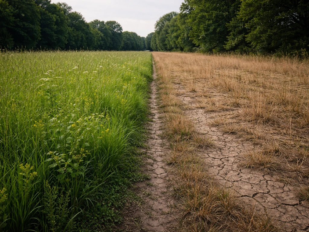
Carrying capacity K is not a fixed number etched into nature. It shifts with conditions. A meadow can support more rabbits in a wet year with abundant grass than in a drought year. A coral reef can support more fish when water temperature stays in the right range. Britannica notes that the geometric or exponential growth of all populations is eventually curtailed by limiting ecological factors, and those factors fall into two broad categories.
- Density-dependent factors: effects that intensify as population density rises. Food competition, disease transmission, waste accumulation, and predator attraction all get worse as more individuals crowd into the same space. These are the primary drivers of logistic regulation.
- Density-independent factors: disturbances that hit populations regardless of how many individuals are present. A hard freeze, a wildfire, or a flood can crash a population whether it numbers 50 or 5,000.
Think of it this way: density-dependent factors are the reason the logistic model works at all. They are the biological mechanism behind the (K - N)/K term. When a population overshoots K temporarily, resources become so scarce that death rates spike and birth rates drop until N falls back toward K. This feedback loop is why real populations oscillate around carrying capacity rather than marching smoothly to it.
Life-history traits, generation time, and r/K thinking
Not all species respond to resource limits the same way. Life-history theory helps explain why a mouse and an elephant, both mammals, behave so differently as populations. The r/K selection framework, though now understood as a spectrum rather than two strict categories, is still a useful thinking tool.
- r-selected species: short generation time, many small offspring, low parental investment, high reproductive rate. They exploit open or disturbed environments rapidly but have high juvenile mortality. Examples: dandelions, mice, most insects, bacteria.
- K-selected species: long generation time, few offspring, high parental investment, low reproductive rate. They are competitive in stable, crowded environments close to carrying capacity. Examples: elephants, whales, oak trees, humans.
Age structure also matters enormously. A population with many young individuals below reproductive age is primed for future growth even if current birth rates look modest. A population skewed toward older individuals may be declining even if it looks numerically large today. Demographers visualize this with population pyramids, but the underlying biology is the same: when individuals reproduce determines how fast N changes, not just how many reproduce.
Generation time directly sets the pace of growth. A bacterium with a 20-minute generation can fill a petri dish overnight. A redwood tree with a generation measured in centuries grows a forest over millennia. When you're working through a population problem, always note the generation time because it sets the timescale on which your model actually applies.
How populations interact with each other and why it changes everything
No population lives in isolation. The growth of one species almost always affects and is affected by others. These interactions add layers of complexity that simple single-species models miss.
Competition
When two species use the same limited resource, both suffer. Intraspecific competition (within a species) is actually the main driver of density-dependent regulation in the logistic model. Interspecific competition (between species) can suppress one or both populations below the K they would reach alone, and in extreme cases can drive a weaker competitor to local extinction through competitive exclusion.
Predation and herbivory
Predator-prey dynamics often generate cyclical population fluctuations. The classic example is the Canadian lynx and snowshoe hare: hare populations boom, lynx numbers follow as food becomes abundant, then hares crash under predation pressure, lynx numbers fall due to starvation, and hares recover to start the cycle again. This oscillation is exactly what you'd expect from two coupled logistic-style populations where one species is both a resource and a regulator for the other.
Symbiosis and mutualism
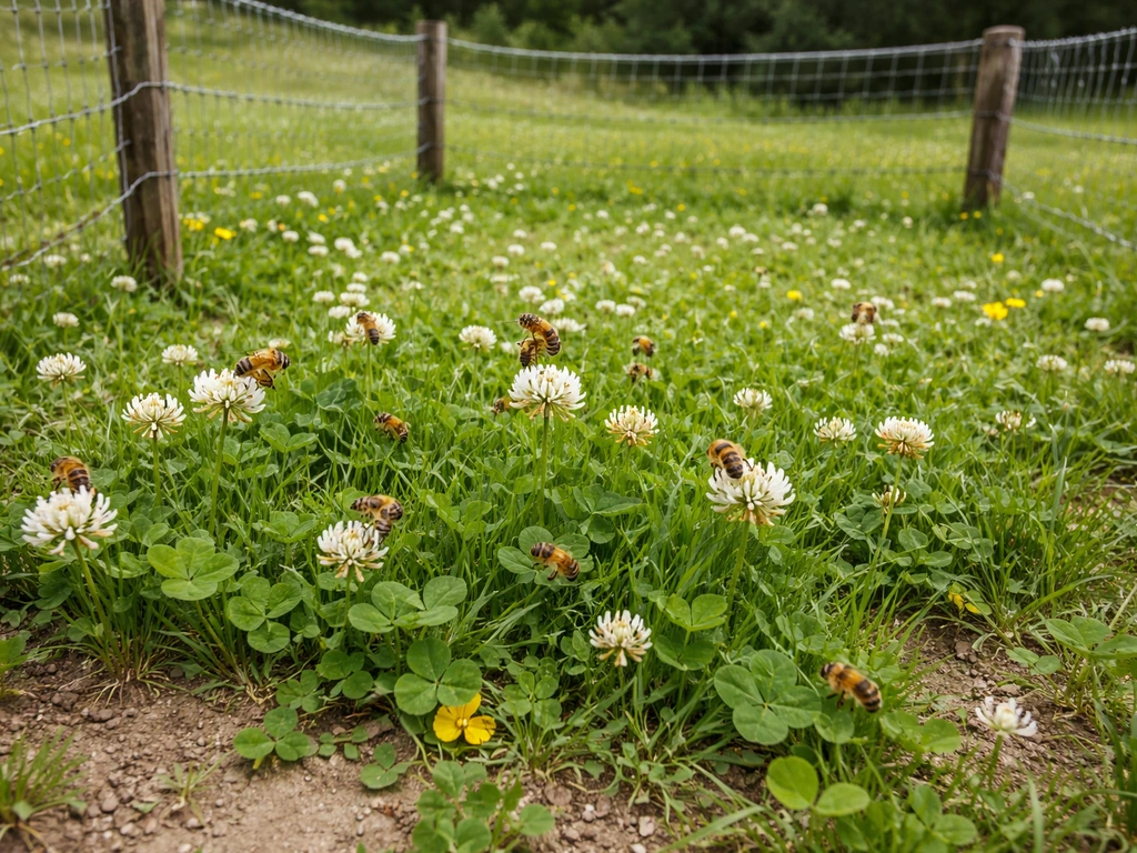
Populations can also help each other grow. Mycorrhizal fungi and plant roots exchange nutrients in a mutualism that can push the effective K of both partners higher than either could achieve alone. Pollinators and flowering plants are another example: more pollinators mean more seeds, more plants mean more nectar, more nectar means more pollinators. These positive feedbacks can accelerate growth well beyond what a single-species model would predict.
Disease and parasitism
Pathogens act as density-dependent regulators with brutal efficiency. Transmission rates rise as individuals crowd together, exactly what the (K - N)/K term captures in aggregate. A disease that spreads easily in a dense population can crash that population well below K almost overnight. This is one reason ecologists watch population density and age structure when modeling disease risk: a dense, immunologically naive population is a pathogen's ideal growth medium.
How to actually analyze or predict population growth
If you need to work through a population growth problem, whether for a biology class, a research project, or genuine curiosity about a local species, here's a practical sequence that works. Family growth depends on many factors like resources, health, and life choices, which can change over time how do families grow.
- Define your population clearly. Specify the species, the geographic boundary, and the time frame. Fuzzy definitions produce meaningless numbers.
- Collect or estimate the four demographic parameters: birth rate (b), death rate (d), immigration rate (i), and emigration rate (e). Even rough estimates matter more than skipping the step entirely.
- Calculate r, the intrinsic growth rate, as r = b - d (for a closed population with no movement). A positive r means the population is growing; negative r means it's declining; r = 0 means it's stable.
- Choose your model. If the population has just colonized an empty habitat with abundant resources, start with exponential growth. If the habitat is established and resources are finite, use logistic growth and estimate K from habitat data, historical peak counts, or resource availability.
- Plug your numbers into the appropriate equation and project forward. For logistic growth, remember that maximum growth rate occurs at N = K/2, which is a useful benchmark: a population at half its carrying capacity is growing fastest.
- Check your assumptions. Is K actually stable, or does it vary seasonally? Are there significant predator, competitor, or disease pressures that the single-species model ignores? If yes, note that your projection is an approximation and flag what direction real dynamics might push it.
- Interpret the output honestly. A model tells you what would happen if your assumptions held. Compare its predictions to observed data and adjust parameters when they diverge.
If you're studying from a textbook and working through structured problems, the answer-key style breakdowns in curriculum materials can help you check whether your parameter choices and equation setups are on track before you apply the reasoning to messier real-world cases. You can practice with chapter-style problems, and then use the chapter 5 lesson 1 how populations grow answer key to verify your calculations.
Putting it all together
Population growth in biology is fundamentally an accounting problem governed by births, deaths, immigration, and emigration. The exponential model describes what growth looks like when nothing limits it, and the logistic model describes what happens when the environment pushes back. Real populations layer on top of those models all the complications of age structure, life-history strategy, and interactions with other species. The (K - N)/K term in the logistic equation isn't just algebra; it represents real mechanisms like food shortage, disease transmission, and competitive pressure that slow growth as populations fill their habitats. Once you see those mechanisms clearly, the math stops being abstract and starts describing something you can actually observe, whether it's bacteria in a flask, deer in a forest, or sourdough starter doubling in a warm kitchen.
FAQ
When I use the population accounting equation, what time window should each term match?
Use N(t+1) = N(t) + B(t) - D(t) + I(t) - E(t) and check that all terms refer to the same time interval. If you only have births and deaths but not movement, you are implicitly assuming I(t)=0 and E(t)=0, which can badly mislead for mobile species like birds, fish, and insects.
How can I tell whether a factor limiting population growth is density-dependent or density-independent?
Density dependence means the growth effects change with crowding, while density independence means they stay roughly the same regardless of N. Weather shocks, for example, can be density independent, while disease transmission often becomes density dependent because contact rates rise as N increases.
Why might a logistic curve not fit a real population even if resources are limited?
The logistic model assumes a stable carrying capacity and a smooth brake on growth. If K is changing quickly (seasonal resources, climate swings, habitat destruction), real trajectories can look like repeated surges and drops rather than a single S-curve.
How does generation time affect interpreting short-term population growth data?
If your study period is shorter than the population’s generation time, you can see little change in N even when reproduction is already underway. In those cases, age structure and time lags can make birth counts look modest while the future increase is still “queued up.”
Can a population decline even when births still occur? (How age structure changes that)
Age structure can reverse the sign of growth compared with what a simple birth rate might suggest. A population with many juveniles about to reproduce can grow even with a currently low average birth rate, while an older-heavy population can decline even if the present birth rate has not yet collapsed.
What does carrying capacity K really represent in practice, beyond “food and space”?
Carrying capacity K is not only about “space.” It aggregates the constraints that limit long-term survival and reproduction, including food availability, shelter, water, nesting sites, and disease pressure. So K can shift when behavior or habitat use changes, not just when weather changes.
How can immigration and emigration make N look stable even when reproduction is not balanced?
Immigration can create growth that exceeds what births alone would predict, especially after a disturbance. Conversely, emigration can mimic low reproduction by exporting individuals, so you should not treat stable N as proof that births balance deaths.
How can I tell from time-series data whether fluctuations are from predator-prey interactions or from logistic self-limitation?
In a predator-prey system, the peak of one population often lags behind the other. If you plot both over time, you may see cycles where prey rise first, predators respond later, then prey crash, then predators crash, which helps distinguish coupling from a single-species logistic pattern.
Why can mutualism speed growth at first but still lead to later crashes?
Mutualisms can effectively raise K, but the boost may not be permanent. If one partner collapses (pollinator declines, disease hits fungi), the mutualistic advantage disappears, and the population can drop sharply.
How does disease change the simple logistic picture of density-dependent regulation?
If a pathogen spreads more efficiently at high density, it can push growth down faster than the logistic brake would predict. Modeling disease often requires adding a transmission or infection state, because deaths from infection can be both density-dependent and time-lagged.
Next Article
Chapter 5 Lesson 1 How Populations Grow Answer Key
Step-by-step answer key for Chapter 5 Lesson 1 population growth: models, graphs, factors, formulas, and why answers fit